01 · Screenshots
Three projections, one platform
The same data — fires, infrastructure, aircraft, GNSS — rendered across 2D flat map, tilted 3D mode, and full globe projection. Basemap switches between dark, OSM, and satellite.
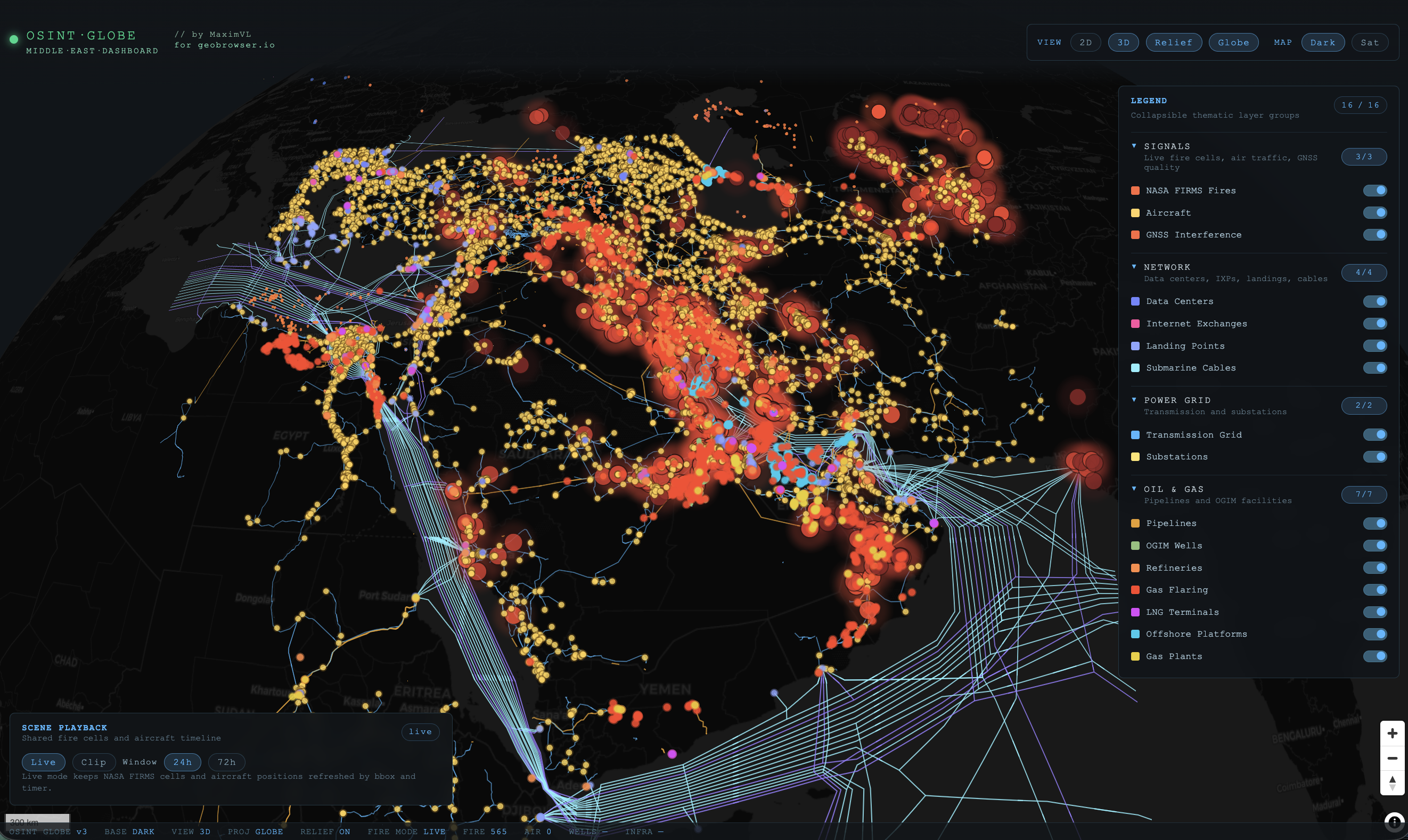
2D · All layers active · Middle East theater
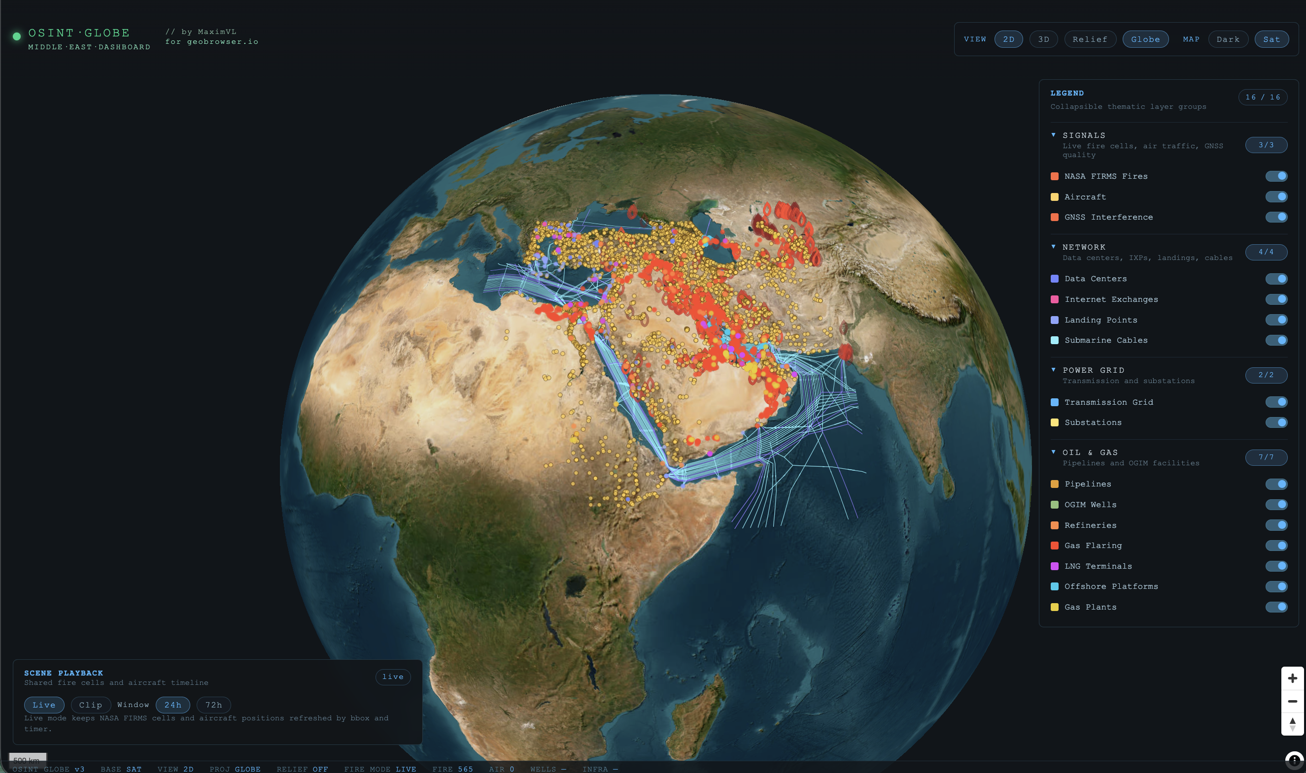
Globe · Satellite basemap
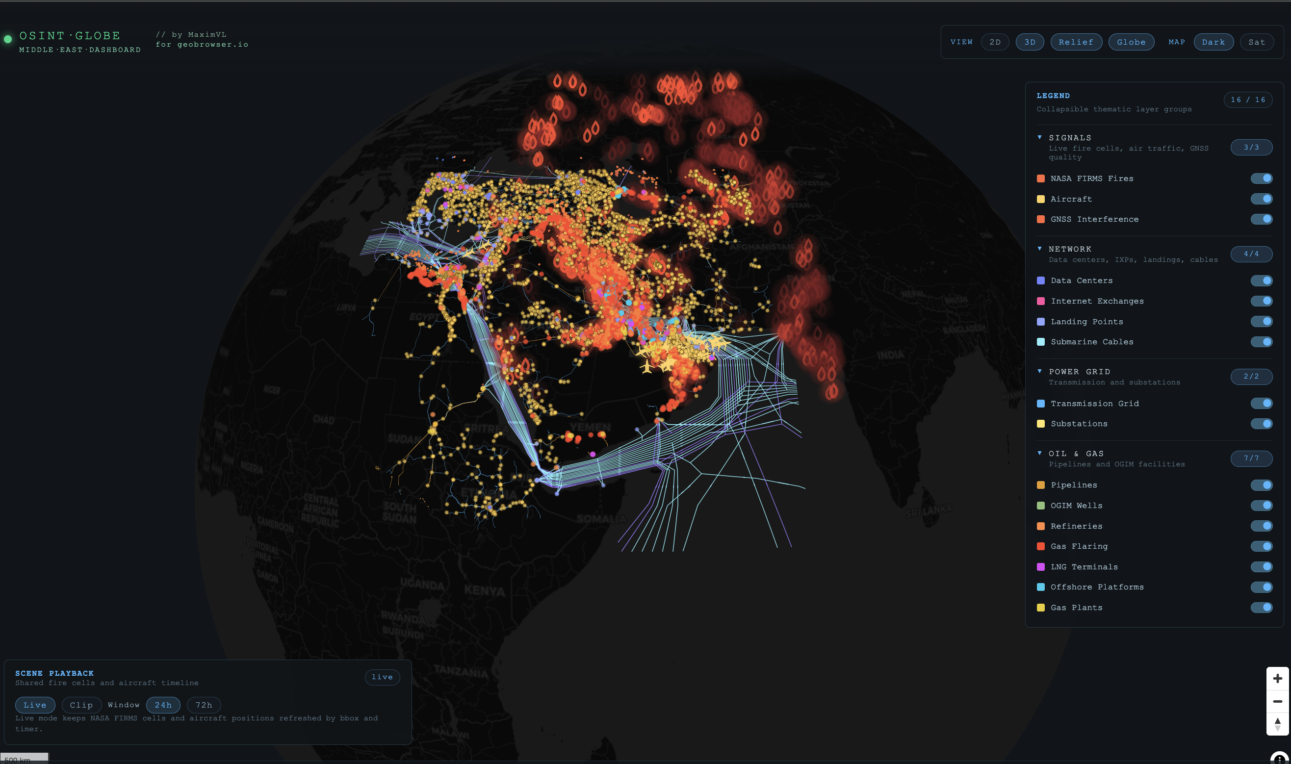
Globe · Dark · Infrastructure overlay
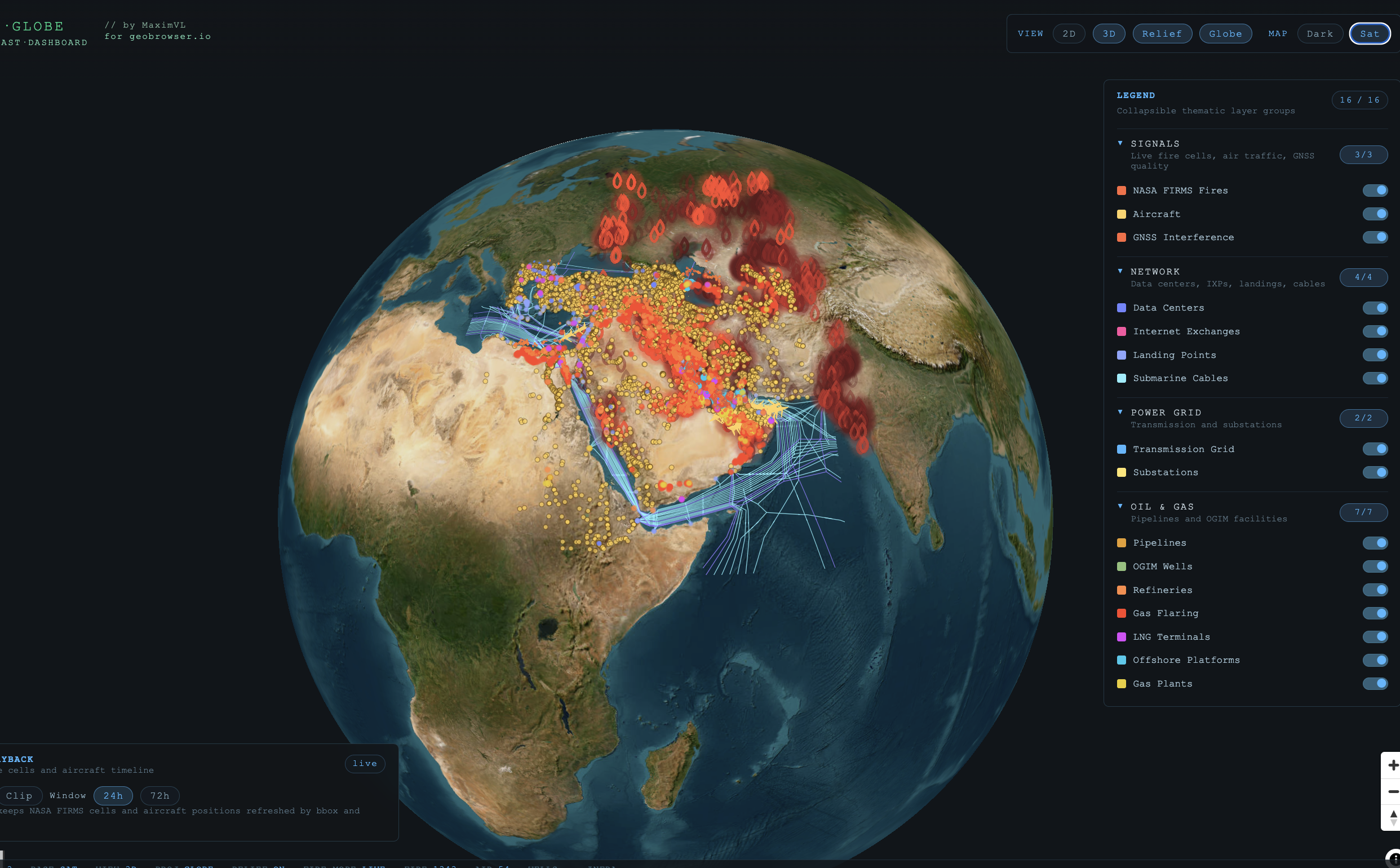
Globe · Satellite · Fire + infrastructure
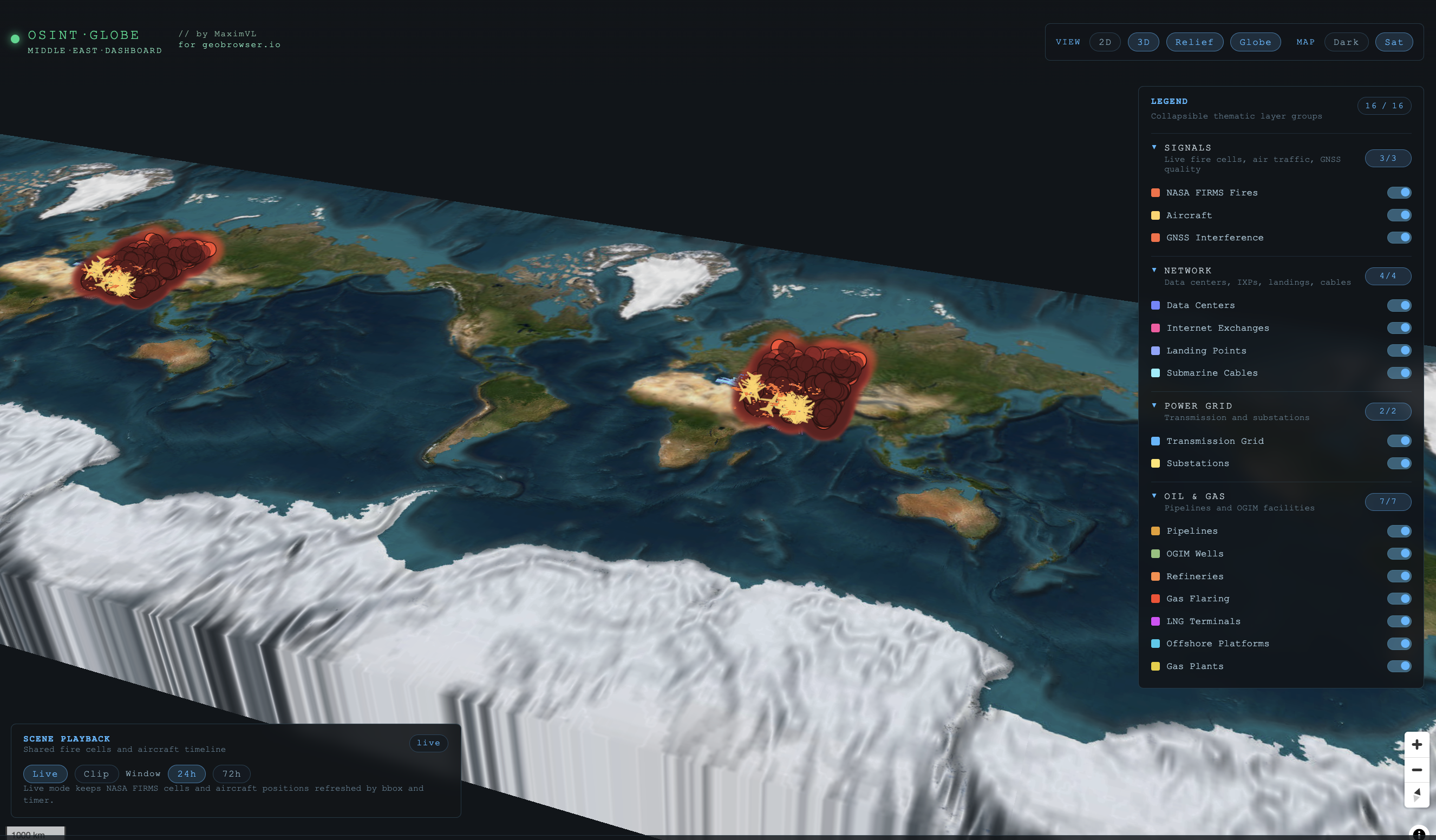
3D · Terrain relief · World view